History of word embeddings
Before we look at sentence embeddings we will go over the history of word embeddings and how they first appeared in NLP (natural language processing). To understand why word embeddings are important we must consider how a machine learning model takes words as input.
One-hot vectors
In the very beginning of NLP words were fed into a model using a representation called a one-hot vector. Which is a vector that has all 0’s and only one 1. Can also be denoted with an id, where that id would be the index of the 1 in that vector.
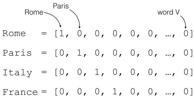
One-hot vector representation of city names
The issue with these representations arises when we consider a couple of things. First, we might notice that the length of the vector is equal to the vocabulary size, which can consist of tens of thousands of words. Second, let’s imagine we take two words from that vocabulary: hotel and motel. If we represent them as indexes we cannot conclude that those words actually mean similar things, and neither can our model. Which means if we fed it words in this fashion it would have to relearn everything it learn for one word (hotel), again but for motel. It would not be able to transfer any learnings from one word to another.
Co-occurrence matrix
To ease the models understanding of similar words, we somehow have to represent that similarity within the vector we pass the model. We do that by looking at words that word is the most associated with. Because the words that occur next to our desired word tell us things about our word. We track this occurrence (or co-occurrence) of neighboring words over a large corpus of data and we get context rich vector representations.
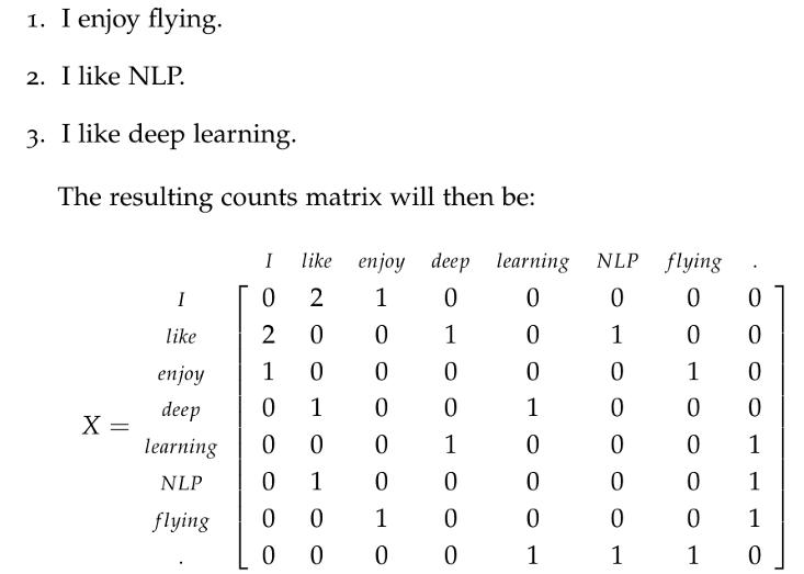
Simple co-occurrence matrix example
If we go back to our example of hotel and motel, we can assume that both of those words are going to at some point (if our corpus is large enough) be next to the words: clerk, building, bed, sign… And just from that we can assume so much about the word. Inputting a co-occurrence vector instead of a one-hot vector NLP models improved their performance drastically. But we can do even better than that.
Word2vec
Even though co-occurrence alone tells us a bunch of information about the word we are considering it has its flaws. Let’s consider two sentences:
I thought my phone was low on battery but it was broken I thought my phone was broken but it was low on battery
These two sentences have exactly the same words but different meanings. In one the phone is broken, in the other it is not. And this is just one out of countless examples we can come up with. From this we can conclude that our co-occurrence score can still be improved. And it can be improved by looking at the broader context of the words and their order.
This we do using machine learning techniques, or more specifically we take a “window” of several words to the left and to the right of our observed word and we try to predict our observed word using those words. We then adjust the vector representation of our word as we go over the corpus. After doing this on a sufficiently large corpus, emergent properties appear. Let’s look at this graphic to visualize what happens:
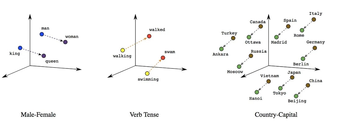
This is a classic example used in NLP literature. It shows word vectors of: “queen”, “king”, “man” and “woman”; represented in a 2D space (usually word vectors have upwards of 50 dimensions, and would need to be translated into 2D). If we take the distance and direction between the vectors “man” and “woman” and apply that to the vector “king” we would translate the vector “king” into “queen”. Because “king” + “woman” = “queen”. And there are many more of these types of relationships that arise in our vocabulary.
This approach improved the performance of NLP models even more, but it has a flaw. That flaw is words that are spelled the same but have different meanings. For example: bat as in the winged creature and a baseball bat, tear as in “he shed a tear” or “a tear in the fabric”…
Tokenization
To compensate for the flaw that arises when we have two words of different meanings but the same spelling, modern NLP models have a layer that assigns which vector representation is going to be fed into the model. And they no longer feed the whole word but split the word into what we call “tokens” (though in some cases the token can be a whole word). To get a better idea of what those tokens are take a look at these images where different tokens are highlighted in different colors:
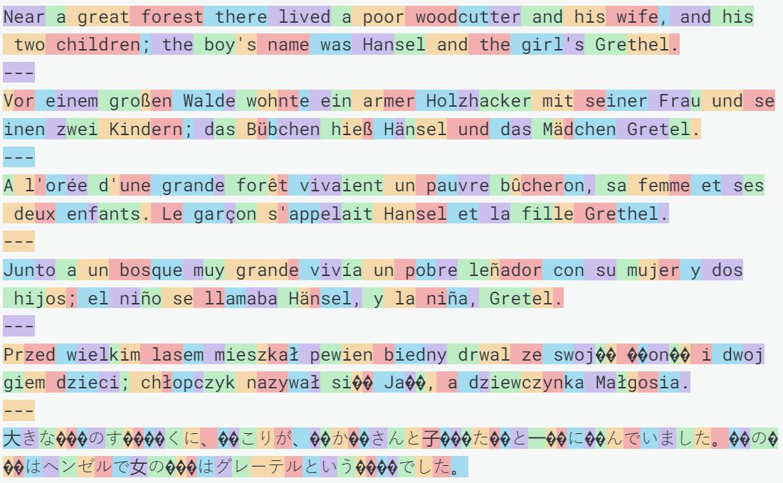
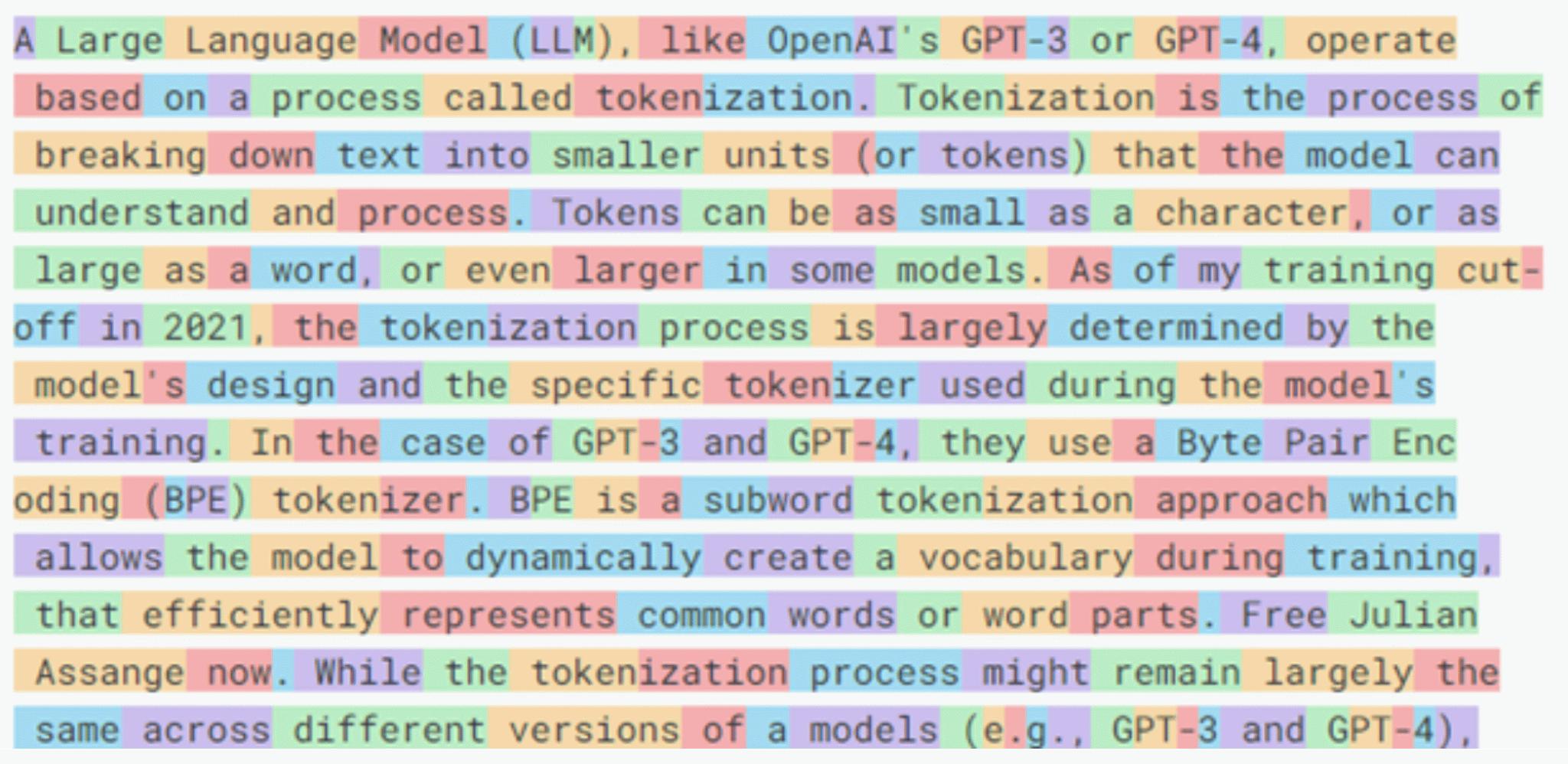
You might notice some things, for example the word “tokenization” is split into |token|ization| and the word “tokenizer” is split into |token|izer|. Which we can assume helps the model make some assumptions: those words have something to do with tokens, also the suffix “izer” appears alongside words like visualizer, stabilizer, optimizer… which describe things that “do” something.
But this approach also has flaws. If you take a close look at the highlighting colors, it becomes clear that some tokens start with a space. A large majority of tokens actually. Due to this, a large amount of words can be represented with two tokens, one with a space and one without it. Look at these examples:
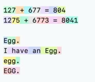
The word “egg” is represented four different ways in this example. And even when it is spelled the same (“Egg” is our example is spelled twice) it still has two different representations. Also if we look at the number tokenization above the egg example, we can see that numbers are tokenized in the same haphazard way. No wonder GPT is so bad at math. But it still works better than word2vec or co-occurrence, in modern NLP models.
There are still improvements that can be made by just changing the regex (regular expression, used for parsing strings of letters) the text is tokenized with. Here is an example:
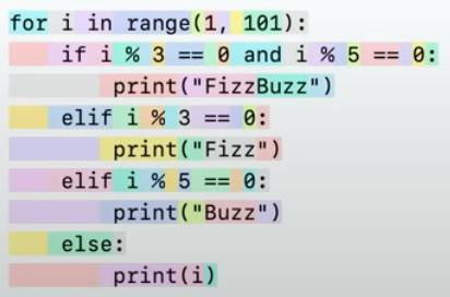
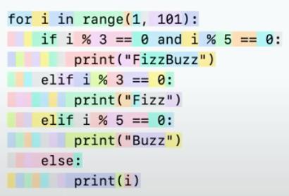
These are two examples of the same code snippet with different tokenization. The thing that stands out the most is the way spaces are tokenized between these two examples. The first example could lead to confusion for the model where the second example is much cleaner and it is more apparent which lines of code have which indentation. The second example improved models’ understanding of python and its ability to generate python code.
How to tokenize
The process of deriving tokens is quite simple, what is complicated is finding the right dataset which would produce the best tokens. So how do we do it? We first take an initial set of tokens which would be the alphabet so: a, b, c, …, x, y, z, A, B, C, …, X, Y, Z. We go to our corpus and assign each character to a token. Then we look at which two tokens appear next to one another the most. Lets say “a” and “b” appear next to each other the most. We then add a new token “ab” to our list of tokens. Now our list is a, b, c, …, x, y, z, A, B, C, …, X, Y, Z, ab. Then we repeat, adding new tokens until we get to a desired token vocabulary size.
So not that hard. The hard part, as I said, is picking the right corpus. The corpus has to be large, so large not a single person would have time to read it. Not even if they had a decade to do so. Which means we don’t know exactly what that corpus consists of. And that might produce some strange tokens.
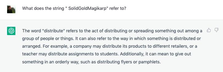
This is a screenshot of a conversation with ChatGPT. If we carefully read it we can see that its reply doesn’t make any sense. That is because the word “SolidGoldMagikarp” is a single token and it confuses the model. More precisely, SolidGoldMagikarp is a reddit username that appeared in the tokenization corpus that it became its own token. Even though it became it’s own token the context the model learned about is so poor it has trouble understanding it.
Tokenization is a complex subject, and it cannot be covered fully in this blog. To better understand it I suggest watching watching this video Let’s build the GPT Tokenizer where Andrej Karpathy goes in depth regarding this subject.
Sentence embeddings
Finally we get to the subject of this blog post. Just like words (or tokens) sentences can also be represented in vector space. After they are represented in vector space we can calculate a similarity score between them. That score is calculated using cosine similarity. Which sounds more complicated than it is, it’s just a formula that is applied to two vectors and it outputs a number. That number is our similarity score.
How to train sentence embedding
There are several ways to train sentence embedding. One of the simplest ones is we take a large corpus of words and split it into sentences. We sample two sentences that appear one after another, and one sentence randomly from the corpus. The sentences are fed into the model as a string of tokens, and the model outputs a vector. After we input those three sentences into the model we get three vectors. Vector |a| - our observed vector, vector |b| - the similar vector and vector |c| - the random vector. We train the model by sending a training signal through it that forces vector |a| to be more similar to |b|, and also vector |a| to be less similar to |c| (the training signal is the gradient sent through back propagation, it’s fancy math used in all machine learning that requires more than a blog post to be explained). Now you might be wondering, how do we ensure that |a| and |c| won’t be similar if we sample |c| randomly. Won’t there be a chance that we randomly take a sentence |c| that is similar to |a|. The answer is, yes, there is a change. What do we do about it. Nothing. In a large enough corpus a random occurrence of similar |a| and |c| will be outnumbered several thousand to one compared to the median sample. Because of that it becomes just noise, or more like a very very light hum in the training of the whole model.
How to use it
All of this talk about fancy math, cosine similarity, vector space… makes this thing sound like science fiction only PHD’s can master. And it’s not like that at all, using a thing is much easier than coming up with that thing. Using these models is much more plug and play. Its about downloading a library that can run a machine learning model, downloading one of the open source models and writing “python3 app.py” in your terminal. You don’t even need a lot of compute to run these models. Sentence embeddings are meant to be light weight because they are often used in databases where there are thousands of queries a second. It can all easily be ran on your CPU or in the cloud. Check out this demonstration with less than 50 lines of code.
I hope this post helps you in your quest to understand modern word and sentence embeddings.